originally posted at https://canmom.tumblr.com/post/101909...
This is the third part in the series about rockets in special relativity!
In this one, we’ll bring everything so far together, and get the details of a mission to another star system. We’ll see how long it takes (for you, and the people you leave behind) and the requirements on your rocket.
OK, so, let’s quickly summarise what we have so far. (Remember that we’re working in units where \(c=1\)!)
In part 1, we showed that when a relativistic rocket changes its speed, the change in speed is related to the change in mass of the rocket by the relativistic rocket equation, $$\Delta v = \tanh \left(v_\text{e} \ln \frac{m_0}{m_1} \right)$$
In part 2, we found the equations for the motion through spacetime of a rocket moving under constant acceleration. As functions of the rocket’s proper time, we found that if the rocket starts at a proper time \(\tau_0\) at a position (\(t(\tau_0),x(\tau_0))\) and velocity \(0\), and accelerates with a proper acceleration \(\alpha\), its motion in an inertial frame is a hyperbola in spacetime given (parametrically as a function of proper time) by \begin{align*}t(\tau)-t(\tau_0)&=\alpha^{-1} \sinh \left( \alpha (\tau-\tau_0) \right)\\x(\tau)-x(\tau_0)&=\alpha^{-1} \left( \cosh \left( \alpha (\tau - \tau_0) \right) -1\right)\end{align*}
Back then we looked at situations where the rocket just accelerates forever, but that’s not all that useful! Such a mission would leave you soaring past your destination near the speed of light, which is not conducive to science.
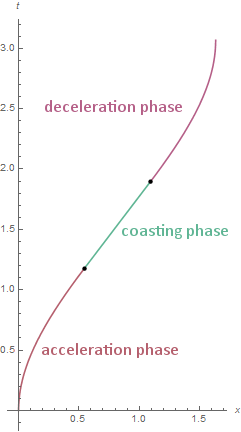
A more sensible approach is to fire your rockets for a while, then perhaps turn them off and coast for a bit to save fuel, and finally when you get near your destination, turn your rocket around and fire the rocket in the opposite direction for the same amount of time, bringing you to a stop.
So we have three phases:
- The rocket starts accelerating at proper time \(\tau=0\) and stops accelerating at a proper time \(\tau = \tau_b\) (b for boost). (Let’s call that the acceleration phase.)
- It flies at a constant speed for a proper duration of \(\tau_c\) (the coasting phase)
- at a proper time \(\tau = \tau_b + \tau_c\), it starts decelerating (accelerating in the opposite direction). It continues decelerating for another proper duration \(\tau_b\) until it comes to a stop at its destination at \(\tau=2\tau_b+\tau_c\) (the deceleration phase).
We should be able to specify a mission with three parameters, then: the acceleration \(\alpha\), the boost duration \(\tau_b\) and the coasting duration \(\tau_c\).
Mission worldline
Right. First thing to do is describe the motion and get some functions \(x(\tau)\) and \(t(\tau)\) for the rocket’s wordline. To do that, we can stitch together the equations for constant velocity motion with the ones for motion under constant acceleration.
Motion at constant velocity \(v\) is pretty simple: just $$x-x_0=v(t-t_0)=\gamma_v v (\tau-\tau_0)$$ (where as before \(\gamma_v=\frac{1}{\sqrt{1-v^2}}\)).
We switch between different kinds of motion at two points: when the rocket stops accelerating at \(\tau=\tau_b\) and when it starts decelerating at \(\tau=\tau_b+\tau_c\). At both of these points, the rocket’s speed and position can’t suddenly change, so \(x(\tau)\), \(t(\tau)\) and \(\frac{\dif x}{\dif t}\) have to be continuous. This allows us to set the parameters for each phase of the flight.
For the acceleration phase, we can use the constant-acceleration solution with \(\tau_0=0\) and (assuming we put the starting point on the origin in the inertial frame we’re using) \(x(\tau_0)=t(\tau_0)=0\). So for \(\tau \le \tau_b\) we’ve got \begin{align*}t(\tau)&=\alpha^{-1} \sinh \alpha\tau \\x(\tau)&=\alpha^{-1} (\cosh \alpha\tau -1)\end{align*}
The coordinate speed at the end of the boost is \begin{align*}\left.\frac{\dif x}{\dif t}\right|_{\tau=\tau_b}&=\left.\frac{\dif x}{\dif \tau}\left(\frac{\dif t}{\dif \tau}\right)^{-1}\right|_{\tau=\tau_b}\\&=\frac{\sinh\alpha\tau_b}{\cosh\alpha\tau_b}\\&=\tanh\alpha\tau_b\end{align*}
That’s really convenient, because (applying the identity \(1-\tanh^2 x = \sech^2 x\)) it implies \(\gamma_v = \cosh\alpha\tau_b\) and \(\gamma_v v = \sinh\alpha\tau_b\).
The coordinate speed in the constant-velocity solution is just the parameter \(v\), so we’ve got to have \(v=\tanh\alpha\tau_b\). So the coasting phase \(\tau_b\lt\tau\le\tau_b+\tau_c\), we have \begin{align*}t(\tau)&=\alpha^{-1} \sinh \alpha\tau_b + (\cosh\alpha\tau_b) (\tau - \tau_b)\\x(\tau)&=\alpha^{-1} (\cosh \alpha\tau_b-1) + (\sinh\alpha\tau_b) (\tau-\tau_b)\end{align*}
This will finish up in a position \begin{align*}t(\tau_b+\tau_c)&=\alpha^{-1} \sinh \alpha\tau_b + \tau_c\cosh\alpha\tau_b\\x(\tau_b+\tau_c)&=\alpha^{-1} \left(\cosh \alpha\tau_b-1\right) + \tau_c\sinh\alpha\tau_b \end{align*}
For the deceleration phase, things can be a bit more complicated. But, because of the symmetry of the situation, we don’t need to work through the equations for hyperbolic motion with an arbitrary starting speed!
We know the rocket must come to a stop at \(\tau=\tau_c+2\tau_b\), so we can use the same equations for hyperbolic motion, this time with \(-\alpha\) instead of \(\alpha\). We can set the spacetime position \((t_\text{stop},x_\text{stop})\) of the stopping point to make the worldline continuous at \(\tau=\tau_b+\tau_c\).
Making the switch from \(\alpha\) to \(-\alpha\), the motion is given by \begin{align*}t(\tau)-t_\text{stop}&=\alpha^{-1} \sinh \left( \alpha (\tau-(2\tau_b+\tau_c)) \right)\\x(\tau)-x_\text{stop}&=-\alpha^{-1} \left( \cosh \left( \alpha (\tau - (2\tau_b+\tau_c)) \right) -1\right)\end{align*}This gives \begin{align*}t(\tau_b+\tau_c)&=t_\text{stop}-\alpha^{-1}\sinh (\alpha \tau_b)\\x(\tau_b+\tau_c)&=x_\text{stop}-\alpha^{-1}\left(\cosh (\alpha \tau_b)-1\right)\end{align*}
As expected, when we set this equal to the position at the end of the coasting phase, we have\begin{align*}t_\text{stop}&=2\alpha^{-1} \sinh \alpha\tau_b + \tau_c\cosh\alpha\tau_b\\x_\text{stop}&=2\alpha^{-1} \left(\cosh \alpha\tau_b-1\right) + \tau_c\sinh\alpha\tau_b \end{align*}
So we’ve got a full solution for the motion of the spaceship: \begin{align}t(\tau) & =\casealign{ & \alpha^{-1} \sinh \alpha\tau & 0\le{}&\tau\lt\tau_b\\&\alpha^{-1} \sinh \alpha\tau_b + (\cosh\alpha\tau_b) (\tau - \tau_b) & \tau_b \le{}&\tau\lt\tau_b+\tau_c\\ & 2\alpha^{-1} \sinh \alpha\tau_b + \tau_c\cosh\alpha\tau_b + \alpha^{-1} \sinh \left( \alpha (\tau-(2\tau_b+\tau_c)) \right) \qquad& \tau_b+\tau_c \le{}& \tau \le 2\tau_b+\tau_c} \\ x(\tau)&=\casealign{ & \alpha^{-1} (\cosh \alpha\tau -1) & 0\le{}&\tau\lt\tau_b \\ & \alpha^{-1} \left(\cosh \alpha\tau_b-1\right) + (\sinh\alpha\tau_b) (\tau-\tau_b) & \tau_b \le{}&\tau\lt\tau_b+\tau_c \\ & 2\alpha^{-1} \left(\cosh \alpha\tau_b-1\right) + \tau_c\sinh\alpha\tau_b -\alpha^{-1} \left( \cosh \left( \alpha (\tau - (2\tau_b+\tau_c))\right) -1\right)\qquad & \tau_b+\tau_c \le{}& \tau \le 2\tau_b+\tau_c}\end{align}
What does that look like?
If we plot that, we get a worldline like this:

That’s the shape we’re expecting: vertical (meaning the rocket is stationary) at the beginning and end of the mission, in the meantime bending towards \(45^{\circ}\) and then away again.
(Note about units: \(x\), \(t\) and \(\tau\) share the same unit since we set \(c=1\). \(\alpha\) is measured in the inverse of that unit.)
OK, let’s have a look at the effects of the different parameters on this shape to see what they all do!
Earlier we found a formula for the duration and distance travelled, \(t_\text{stop}\) and \(x_\text{stop}\): \begin{align*}t_\text{stop}&=2\alpha^{-1} \sinh \alpha\tau_b + \tau_c\cosh\alpha\tau_b\\x_\text{stop}&=2\alpha^{-1} \left(\cosh \alpha\tau_b-1\right) + \tau_c\sinh\alpha\tau_b \end{align*}From that we expect both to be linear in \(\tau_c\), and depend on the other parameters in a more complicated way.
Keeping the boost durations the same (both set to 1 unit) but varying acceleration gives this effect:
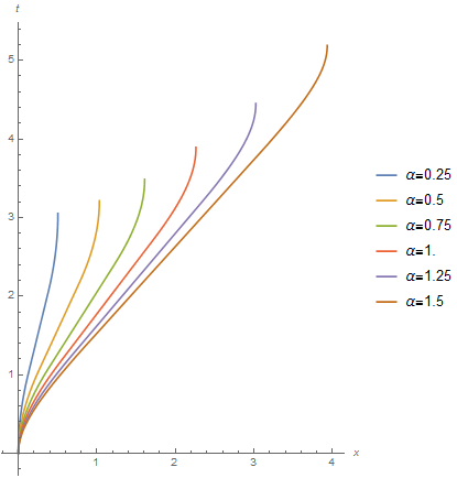
As we’d expect, increasing the acceleration gets you closer to the speed of light and therefore takes you further in the same proper time. Because of time dilation, although all these missions have the same proper time, they take different amounts of coordinate time.
OK, what about if we vary \(\tau_b\) while keeping \(\alpha\) and \(\tau_c\) constant (each set to 1)?
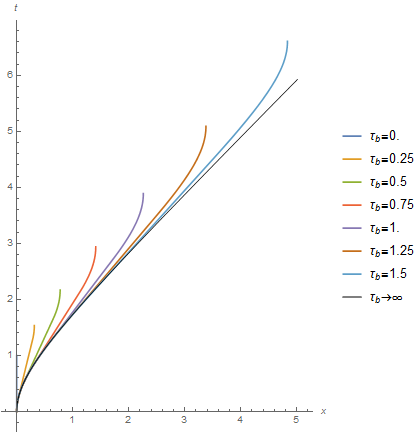
We can see that these seven worldlines are all the same to begin with, and the boost time determines where they break away from the endless-acceleration hyperbola (the black line marked \(\tau_b\to\infty\)).
We can also see that both the coordinate time to reach the destination and the total distance travelled increase nonlinearly with \(\tau_b\).
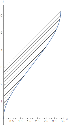
OK, finally, let’s try this with \(\tau_c\), keeping \(\alpha\) and \(\tau_b\) as 1.

This time, the worldlines are the same until each one reaches its deceleration phase. As expected, the distance travelled and the coordinate duration is linear in \(\tau_c\).
Messages from Earth and redshift
In the last post, we saw how a rocket that accelerates forever has an event horizon, meaning it won’t ever receive any messages from Earth that were sent a certain point after it left (about a year if it’s accelerating at \(g\)).
What happens to messages from Earth this time? Let’s imagine someone on Earth sends regular radio messages out towards the rocket. Each one travels at the speed of light, so it will make a \(45^{\circ}\) line on the spacetime diagram.
One clear thing: the arrivals of the messages get increasingly spaced apart on the spaceship’s worldline, which is pretty suggestive that the messages will seem to be spread out in time to the ship. This will be further exarcerbated by time dilation.
Just how much?
If Earth sends a message at Earth time \(t_0\), each line’s equation will therefore just be \(x=t-t_0\). To figure out the value of \(\tau\) when the message arrives, we need to solve that with the equations for the spaceship’s wordline.
For the acceleration phase, we have $$\alpha^{-1}(\cosh\alpha\tau-1)=\alpha^{-1}\sinh\alpha\tau-t_0$$ so \(\cosh\alpha\tau-\sinh\alpha\tau=1-\alpha t_0\). From the definitions of \(\cosh\) and \(\sinh\), we have \(\cosh x - \sinh x = \exp (-x)\), implying \(\tau=-\alpha^{-1}\ln(1-\alpha t_0)\).
(When \(t_0 \gt \alpha^{-1}\), there’s no solution for \(\tau\), confirming there’s an event horizon if you accelerate forever.)
This stops being valid at \(\tau=\tau_b\), i.e. for messages sent after \(t_0=\alpha^{-1}(1-\exp (-\alpha\tau_b))\). After that we need to use the solution for the coasting phase, so $$\alpha^{-1} (\cosh \alpha\tau_b-1) + (\sinh\alpha\tau_b) (\tau-\tau_b)=\alpha^{-1} \sinh \alpha\tau_b + (\cosh\alpha\tau_b) (\tau - \tau_b)-t_0$$We can immediately make the same simplification: $$\alpha^{-1} (\exp(-\alpha\tau_b)-1)=(\exp(-\alpha\tau_b))(\tau-\tau_b)-t_0$$ so along this part of the worldline, $$\tau=\alpha^{-1}(1-\exp \alpha\tau_b)+\tau_b+t_0 \exp \alpha\tau_b$$
To check this, we can insert \(t_0=\alpha^{-1}(1-\exp (-\alpha\tau_b))\) to make sure it gives \(\tau=\tau_b\). (It does.)
That stops being valid when \(\tau=\tau_b+\tau_c\), at which point it’s receiving messages from \(t_0=\alpha^{-1}(1-\exp(-\alpha\tau_b)) +\tau_c \exp (-\alpha \tau_b) \). Now onto the deceleration phase… (This is getting incredibly tiring, but we’re nearly done.)
Proceeding similarly to the last two cases for the deceleration phase gets us\begin{align*}2\alpha^{-1} (\cosh \alpha\tau_b-1) + \tau_c\sinh\alpha\tau_b -\alpha^{-1} \Big( \cosh \big( \alpha (\tau - (2\tau_b+\tau_c))\big) -1\Big)&\\=2\alpha^{-1} \sinh \alpha\tau_b + \tau_c\cosh\alpha\tau_b + \alpha^{-1} \sinh \big( \alpha (\tau-(2\tau_b+\tau_c))\big)-t_0&\end{align*}
Simplifying that in the same way in a few steps… \begin{gather*}2\alpha^{-1}(\exp(-\alpha\tau_b)-1)=\tau_c \exp(-\alpha\tau_b)+\alpha^{-1}\Big(\exp\big(+\alpha(\tau-(2\tau_b+\tau_c))\big)-1\Big) -t_0\\\exp\big(+\alpha(\tau-(2\tau_b+\tau_c))\big)=\alpha t_0 -1 + (2-\alpha\tau_c)\exp(-\alpha\tau_b) \\ \tau=2\tau_b+\tau_c + \alpha^{-1} \ln \big(\alpha t_0 - 1 + (2-\alpha \tau_c)\exp(-\alpha\tau_b) \big)\end{gather*}
To check this, we put \(t_0=\alpha^{-1}(1-\exp(-\alpha\tau_b)) +\tau_c \exp (-\alpha \tau_b) \) in there to see if you get \(\tau=\tau_b+\tau_c\). (And everything seems to be in order…)
That leaves us with the following relationship between the time \(t_0\) a message is sent and the proper time \(\tau_r\) when it reaches the spaceship: $$\tau_r(t_0)=\casealign{ & -\alpha^{-1}\ln(1-\alpha t_0) & 0 \le {} & t_0 \lt \alpha^{-1}(1-\exp (-\alpha\tau_b)) \\ & \alpha^{-1}(1-\exp \alpha\tau_b)+\tau_b+t_0 \exp \alpha\tau_b & \alpha^{-1}(1-\exp (-\alpha\tau_b)) \le {} & t_0 \lt \alpha^{-1}(1-\exp(-\alpha\tau_b)) +\tau_c \exp (-\alpha \tau_b) \\ & 2\tau_b+\tau_c + \alpha^{-1} \ln \big(\alpha t_0 - 1 + (2-\alpha \tau_c)\exp(-\alpha\tau_b) \big) \qquad & \alpha^{-1}(1-\exp(-\alpha\tau_b)) +\tau_c \exp (-\alpha \tau_b) \le {} & t_0 < 2\alpha^{-1}(1 - \exp(-\alpha \tau_b)) + \tau_c \exp(-\alpha \tau_b)}$$
OK, but what does that mean?
Let’s plot it! (Here with \(\alpha\), \(\tau_b\) and \(\tau_c\) set to 1.)
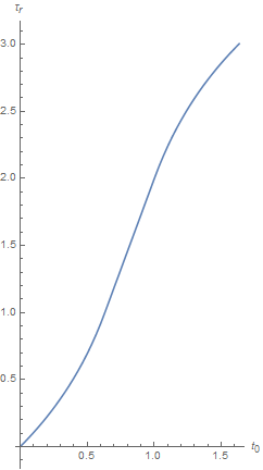
When the rocket is not moving relative to the Earth, this plot is a straight \(45^\circ\) line. However, as the rocket accelerates, the line becomes steeper! That means a short interval of time on Earth represents a much longer time on the spaceship.
This also applies to things like electromagnetic waves! This is the cause of relativistic doppler shift; the messages from Earth won’t just arrive less frequently, but the waves themselves will have a lower frequency too (so visible light becomes more red).
That is a fairly mild example. Let’s double \(\alpha\), \(\tau_b\) and \(\tau_c\).
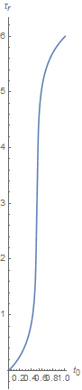
The graph looks almost vertical! Which means that that tiny instant on Earth will be dragged out over a huge amount of time on the spaceship.
Mass ratios
How do we pick out the parameters? We’re limited by the design of our spaceship: the mass ratio and exhaust velocity.
The change in coordinate velocity during the acceleration phase is (in natural units) \(v=\tanh\alpha\tau_b\), so the rocket equation for this boost gives us $$\tanh\alpha\tau_b=\tanh \left(v_\text{e} \ln \frac{m_0}{m_1} \right)$$which implies the simple relationship$$\alpha\tau_b=v_\text{e}\ln\frac{m_0}{m_1}$$which is actually just like the Newtonian case. This means the mass ratio for this boost is $$\frac{m_0}{m_1}_\text{boost}=\exp \left(\frac{\alpha\tau_b}{v_\text{e}}\right)$$We have to do this twice, so the mission’s total mass ratio is the square of this, i.e. $$\frac{m_0}{m_1}=\exp\left(\frac{2\alpha\tau_b}{v_\text{e}}\right)$$
(Why have I argued this in this funny one-boost-at-a-time order? Because of the complications in combining the velocities of two boosts in opposite directions in special relativity, this way seems less likely to make a mistake.)
Putting some real numbers in
If we want to know how long actual space missions will take, we need to restore \(c\). We do this pretty much by staring at the dimensions and going ‘hmm’ then putting in \(c\) until all the dimensions are right.
That leaves us with the following values to fully describe a space mission:\begin{align*}t_\text{stop}&=2\frac{c}{\alpha} \sinh \frac{\alpha\tau_b}{c} + \tau_c\cosh\frac{\alpha\tau_b}{c}\\x_\text{stop}&=2\frac{c^2}{\alpha} \left(\cosh \frac{\alpha\tau_b}{c}-1\right) + c\tau_c\sinh\frac{\alpha\tau_b}{c}\\\tau_\text{stop}&=2\tau_b+\tau_c\\\frac{m_0}{m_1}&=\exp\left(\frac{2\alpha\tau_b}{v_\text{e}}\right)\\v_\text{max}&=c\tanh\alpha\tau_b \end{align*}
What can we do with this? An awful lot! We put in the things we know, and then see what that implies about the remaining parameters.
Boosting to Alpha Centauri
For example, suppose we want to go to Alpha Centauri, which is 4.4 light years away, so we have \(x_\text{stop}=4.4c \unit{ y }\). Fortunately, we have an antimatter rocket with an effective exhaust velocity of \(v_\text{e}=0.6c\)!
Let’s also imagine our spaceship accelerates at a very human-comfortable \(g\), and we don’t bother with a coasting phase (which lets us rely on our acceleration to provide a sensation of gravity for the entire trip) so \(\tau_c=0\).
With these assumptions, we can calculate the rest of the quantities. First,$$4.4\unit{y}c=\frac{2c^2}{g}\left(\cosh \frac{g\tau_b}{c} -1\right)$$ so $$\tau_b=\frac{c}{g}\arccosh\left(\frac{2.2\unit{y}g}{c}+1\right)\approx1.8\unit{y}$$which Wolfram Alpha helpfully informs me is the gestation period of an elephant. From that, we can quickly find that the coordinate duration of the mission is \(t_\text{stop}=6\unit{y}\), the proper duration of the mission is \(\tau_\text{stop}=3.6\unit{y}\), and the mass ratio for the mission is around 484. (The Apollo missions had a mass ratio of 36, so this is pretty silly).
Let’s check the Valkyrie
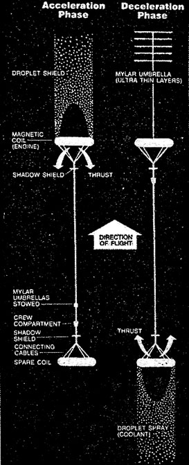
One of my favourite spaceship designs is the Valkyrie (which I heard about on Atomic Rockets), a speculative design by Charles Pellegrino with help from some scientists Jim Powell, Hiroshi Takahashi and Pierre Noyes.
The really cool idea is that the spaceship’s payload can be towed 10km behind its engines instead of pushed from the back, which means you don’t need loads of heavy compressive elements.
Their mission is very like the one we’ve described. Instead of turning around, at the end of the coasting phase, the crew compartment moves to the other end of the line, and another engine at the back of the spaceship turns on to decelerate them.
The Valkyrie mission is a bit more complicated than what we’ve examined here, initially using higher-acceleration but lower exhaust velocity antimatter-triggered fusion, and gradually switching to pure proton-antiproton annihilation. It also doesn’t turn the engines off entirely during the coasting phase, but leaves them on at a much smaller acceleration to keep the line taut and maintain their droplet shield to protect from space dust.
We know the maximum attained speed is \(c\tanh\frac{\alpha\tau_b}{c}=0.92c\). We also know the mass ratio is \(\frac{m_0}{m_1}=\exp\left(\frac{2\alpha\tau_b}{v_\text{e}}\right)=22\).
The first equation tells us that \(\alpha\tau_b=c\arctanh 0.92\), and with the second we have $$v_\text{e}=\frac{2c\arctanh 0.92}{\ln 22}\approx c$$which shows us they were assuming an effective exhaust velocity very close to \(c\)…
Apparently this is good for getting you up to 12 light years away in a reasonable amount of proper time, so let’s set \(x_\text{stop}=12\unit{y}c\). This implies $$\tau_c=\frac{0.43c}{\alpha}(12\unit{y}\alpha-3.1)$$
We can’t go much further without a value for the acceleration. During the coasting phase, the front engine apparently provides \(10^{-5}g\), but frustratingly the websites don’t seem to mention what the acceleration is used during the acceleration and deceleration phases. If we assume it’s \(g\), the coasting phase lasts \(\tau_c=3.8\unit{y}\) and the boost phases each last \(\tau_b=1.5\unit{y}\), so the total proper time is \(6.9\unit{y}\). The coordinate time elapsed is about \(14.3\unit{y}\).
Judging by the comments about the direct proton-antiproton annihilation having a low thrust despite its high exhaust velocity, I suspect \(g\) is a little bit high. Still. It seems like their calculations are plausible!
OK, that’s it!
The world line expressions, alongside those five equations up there, are a detailed description of a plausible space mission. I am… really quite proud of that :p
As you can see from the examples, though, they’re rather fiddly to use in practice. It would be nice if we could make some kind of space mission calculator, a web page which lets you set some of the values and calculate the rest. Better yet, a computer can let you stack up an arbitrary series of mission phases without doing all this algebra.
Mathematica should be capable of that relatively easily! Which is all well and good, as long as I can persuade people to download the Wolfram CDF Player.
Otherwise, doing it in Python or even Javascript shouldn’t be impossible, though it would take rather more thought and studying. (It’s funny: the internet is littered with somewhat broken calculators for esoteric subjects. Now it’s my turn to make one…)
The other thing I’m going to do is make some animations, and a much more readable, accessible summary with fewer derivations and less of a blizzard of equations. And I’ll be extremely happy to answer any questions people have, or extra ideas or whatever. Otherwise, that’s it!
Comments
noda
hope you are still working the above calculator. these posts are really well written!